





bladeRF xA4 or xA9 for Custom FPGA DSP? Comparing Resource Use and Timing
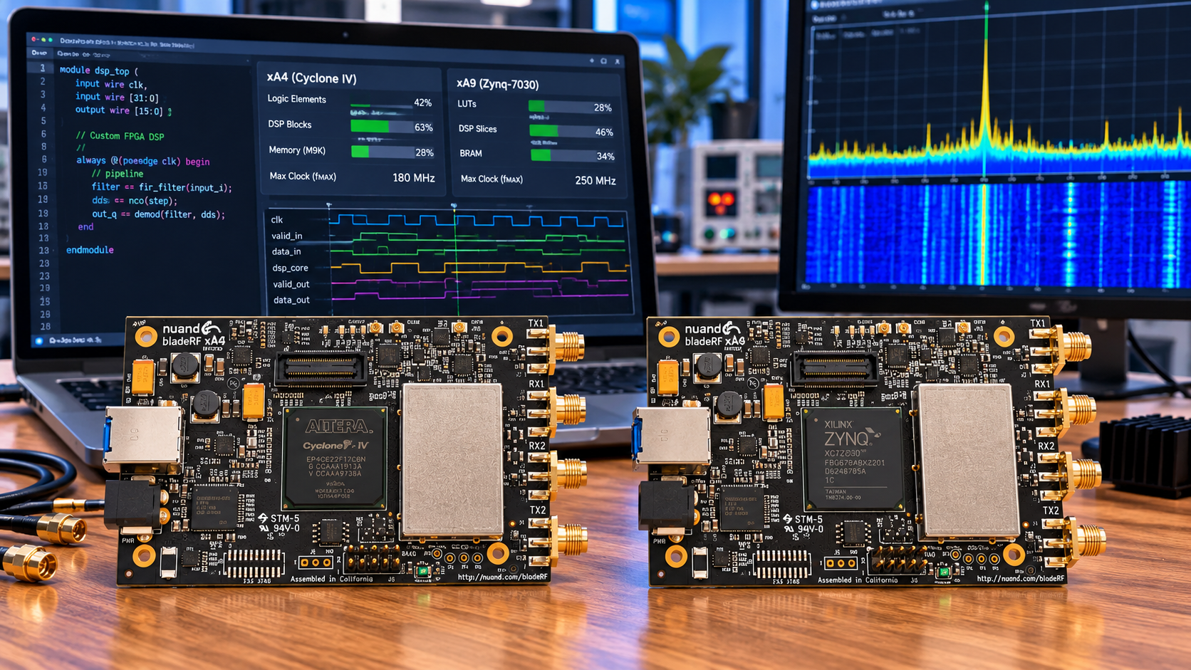
Choose bladeRF xA4 when your custom DSP fits alongside the required platform logic with acceptable timing and margin. Choose xA9 when the design needs substantially more logic, memory or multipliers, or when an established roadmap justifies that room. A bigger FPGA does not automatically improve RF sensitivity or make an unpipelined design run faster.
Our bladeRF 2.0 micro xA4 and xA9 share the platform's RF and USB architecture. The purchase decision for custom HDL should follow an implementation budget rather than a generic “more powerful” label.
Compare the published FPGA resources
| Resource | xA4 | xA9 |
|---|---|---|
| Logic elements | 49 kLE | 301 kLE |
| FPGA memory | 3,383 kbits | 13,917 kbits |
| Variable-precision DSP blocks | 66 | 342 |
| Embedded 18 × 18 multipliers | 132 | 684 |
These are total resources from Nuand's platform specification. DSP-block and multiplier counts describe related capabilities of the same hardware; do not add them as independent processing pools. Mapping also changes with operand width and DSP operating mode.
Not all resources are available to your algorithm. The host interface, radio control, clocks, buffering and other platform functions consume part of the device. Published approximate free-logic figures depend on the baseline image and are not a guaranteed budget for your exact build.
Start with a baseline compile
Pin the bladeRF HDL revision and use the supported FPGA toolchain for that revision. Build the unmodified target for the exact xA4 or xA9 device, then save the synthesis, fitting and timing reports. This gives a realistic reference for incremental resource use.
The official FPGA development guide explains the platform and sample paths. Some examples also discuss older bladeRF hardware. Select the bladeRF 2.0 micro target and matching files instead of copying a classic-board command without checking it.
Record clock frequencies, reset arrangements, available sample interfaces and any assumptions about backpressure. A filter that produces the right values in isolation still needs correct integration with the radio's streaming system.
Budget operations before counting multipliers
Consider an illustrative 32-tap real-coefficient FIR applied separately to I and Q. One complex stream needs 64 real multiplications per output sample in a straightforward implementation. Two such streams need 128. At 10 MS/s per stream, the total arithmetic rate is 1.28 billion real multiplications per second.
That does not necessarily mean 128 physical multipliers. An idealised 100 MHz processing engine has ten clock cycles per 10 MS/s sample period and may time-share arithmetic. Coefficient symmetry, polyphase structures and operand widths can change the mapping further.
This calculation is a design exercise, not a measured bladeRF implementation. Control overhead, memory access, routing and achievable clock frequency determine whether the intended sharing scheme works.
Memory and data movement can decide the board
FFT buffers, long correlation windows and channel histories can exhaust memory before logic. Calculate stored samples from the actual width. For example, 4,096 complex samples at 16 bits per component require 131,072 bits, or 16 KiB, before metadata and buffering overhead.
Double buffering doubles that storage. Multiple channels and simultaneous processing stages multiply it again. FPGA memory is also organised into finite blocks with port and width restrictions, so allocated memory can exceed the raw bit calculation.
When processing reduces data before USB transfer, specify the output representation and host changes. Adding an accelerator does not automatically reduce USB traffic unless it changes what is sent or where processing occurs.
Resource fit and timing closure are different checks
A design can use fewer than the available logic elements and still fail timing because a path is too long or routing is congested. At an illustrative 100 MHz clock, the period is 10 ns; the usable data-path budget also includes clock and register timing requirements.
Pipeline arithmetic, plan fanout and memory access, and review every relevant clock domain. Check setup and hold requirements, clock-domain crossings and unconstrained paths. A positive slack number is not useful if a critical path was accidentally excluded.
Compare routed results for the actual device and constraints. xA9 offers room for parallelism and buffering, but its larger fabric does not provide a universal clock-speed advantage. Do not promise a percentage speedup from the resource table.
Define the evidence needed to choose
- A baseline platform build and the same build with your DSP added.
- Incremental logic, DSP and memory use, with the selected tool version.
- Worst-case timing reports and a review of constraints and crossings.
- Simulation against a software reference, including rounding, saturation and overflow.
- Continuous sample tests at the intended rates and channel counts.
- Latency accounting for pipelines, FIFOs and host buffering separately.
For example, 60 pipeline cycles at 100 MHz contribute 0.6 microseconds. That excludes FIFO waiting, radio conversion and host scheduling. State the measurement boundary before advertising latency.
Match the model to the project
xA4 is a sensible candidate for learning, modest filters, detectors and primarily host-based GNU Radio work. xA9 is the stronger candidate when large FFTs, correlators, modem stages or several processing chains create a demonstrated resource requirement.
Nuand states that the platform does not ship with the custom accelerators described as possible applications. Your team must design or obtain the HDL and integrate it. Buying xA9 is buying capacity, not a finished DSP application.
Frequently asked questions
Does xA9 receive better than xA4?
The FPGA size is not an RF sensitivity upgrade. Choose it for digital implementation needs.
Can I load an xA9 image on xA4?
No. Build or obtain the image for the exact FPGA target.
Is synthesis enough to prove performance?
No. Routing, timing analysis and continuous operation on hardware are necessary checks.
Should I choose xA9 before the DSP design exists?
It may be justified by a documented roadmap, but make that a capacity allowance rather than a claim of demonstrated need.
Read our general xA4/xA9 comparison, then use Add to Quote with the chosen model and any enclosure, cable or reference requirements.
No posts found
Write a review






We support all major card and digital payment options. More local methods are available and shown during checkout.
You enter into a binding sales contract once you have received an 'order confirmation and sales receipt' email from us, in line with our Sales & Delivery conditions. Therefore, sdrstore.eu has the right to cancel your order in the event of technical problems, delivery failure, Fair use policy and other similar situations.






Your payments are protected by advanced encryption and 3-D Secure authentication for safe online shopping.