+3197010267156

Home/SDRstore.eu Blog | SDR, Electronics & Tech Guides/NanoVNA Setup Guide: Calibration, SWR, Smith Chart, and Antenna Testing

SDRstore.eu • 06/03/2026

NanoVNA Setup Guide: Calibration, SWR, Smith Chart, and Antenna Testing

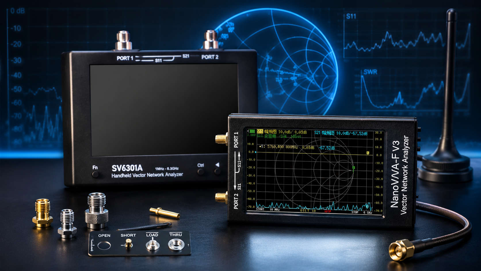
A NanoVNA is one of the most useful tools you can add to an RF toolkit. It can help you test antennas, find the resonant frequency of a whip or dipole, check SWR across a band, view impedance on a Smith Chart, measure filter response, and identify problems in cables or RF components.

The device is affordable and portable, but accurate results depend on using it correctly. A NanoVNA is not a plug-and-read meter. You need to select the right frequency range, calibrate the device at the correct reference plane, use the correct port, and understand what the traces actually mean.

This NanoVNA setup guide explains calibration, SWR, the Smith Chart, antenna testing, markers, common mistakes, and the best beginner workflow. It is written for radio hobbyists, Meshtastic users, antenna builders, SDR enthusiasts, CB users, amateur-radio operators, and anyone learning RF measurements.

To compare available models, browse the spectrum analyzers and RF analysis tools at SDRstore.eu.

Quick Answer: How Do You Test an Antenna with a NanoVNA?

The basic NanoVNA antenna-testing workflow is:

Disconnect the antenna from any transmitter, radio, amplifier, or powered device.
Set the NanoVNA start and stop frequencies around the band you want to test.
Attach the cable or adapter you plan to use.
Calibrate CH0 using the Open, Short, and 50-ohm Load standards.
Set one trace to CH0 SWR.
Optionally set a second CH0 trace to Smith Chart or LogMag.
Connect the antenna to CH0, also called Port 1.
Use a marker to locate the lowest SWR point.
Adjust the antenna length or matching network in small steps.
Recheck the full operating band before using the antenna with a radio.

If the SWR dip appears below your intended frequency, the antenna element is generally too long. If the dip appears above the intended frequency, the antenna element is generally too short.

What Is a NanoVNA?

NanoVNA is a compact vector network analyzer. A VNA sends a controlled RF signal into a device and measures what is reflected back or what passes through.

That sounds technical, but the beginner use cases are straightforward:

Check whether an antenna is matched correctly.
Find the frequency where an antenna performs best.
Measure SWR across an amateur-radio, CB, LoRa, Meshtastic, Wi-Fi, GPS, or other RF band.
View antenna impedance and reactance.
Test filters, attenuators, cables, and RF components.
Measure insertion loss through a device.
Use TDR features on supported models to investigate cable length or cable faults.

A NanoVNA does not directly measure antenna gain, radiation pattern, or real-world range. It tells you how the antenna or RF system behaves electrically at its connector. That is extremely useful, but it is only part of complete antenna performance.

NanoVNA Ports Explained: CH0 and CH1

Most NanoVNA models have two SMA ports. Choosing the correct port is essential.

Port	Common Label	Measurement Type	Use It For
Port 1	CH0, TX, Reflect, or S11	Reflection measurement	Antenna SWR, impedance, return loss, and Smith Chart testing
Port 2	CH1, RX, Through, or S21	Transmission measurement	Filter response, insertion loss, cable loss, attenuators, and RF components

For normal antenna testing, connect the antenna only to CH0. You do not need CH1 unless you are measuring how a signal passes through a component.

Safety First: Protect Your NanoVNA

A NanoVNA is a measurement instrument with sensitive RF inputs. Do not connect it to an active transmitter or a cable that may carry RF power.

Before connecting an antenna:

Disconnect the antenna from all radios and transmitters.
Turn off amplifiers, bias-tee power, and active equipment unless your exact test requires them and you understand the limits.
Safely discharge static from outdoor antenna feedlines before connecting the NanoVNA.
Do not connect unknown RF sources directly to the VNA.
Use attenuation or proper RF protection when testing active equipment.
Avoid overtightening SMA connectors.

Outdoor antennas can accumulate static charge from wind and weather. Discharge the feedline safely according to your installation practices before connecting sensitive test equipment.

What Comes in a NanoVNA Calibration Kit?

Most NanoVNA packages include small SMA calibration standards. These are not optional accessories. They are required for accurate measurements.

Calibration Standard	Purpose	Used For
Open	Creates an open-circuit reference	One-port calibration on CH0
Short	Creates a short-circuit reference	One-port calibration on CH0
Load	Provides a 50-ohm reference load	One-port calibration on CH0
Through adapter or barrel	Connects CH0 directly to CH1	Two-port S21 transmission measurements

Antenna testing normally needs Open, Short, and Load calibration on CH0. Filter and cable measurements normally add the Through step between CH0 and CH1.

The Most Important Rule: Set the Frequency Range Before Calibration

Calibration is valid only for the sweep range you selected. Set the start and stop frequencies first. Then calibrate.

If you calibrate from 100 MHz to 200 MHz and later change the sweep to 400 MHz to 500 MHz, the old calibration should not be trusted. Recalibrate after changing the frequency span.

Recommended workflow

Choose a broad sweep range to locate the antenna resonance.
Calibrate for that broad range.
Find the approximate SWR dip.
Narrow the sweep around your target operating band.
Recalibrate for the narrower range.
Make the final antenna adjustments using the narrower sweep.

A narrow sweep gives a more useful graph for fine tuning because small frequency changes become easier to see.

Reference Plane Explained: Where Should You Calibrate?

Calibration tells the NanoVNA where the measurement starts. This location is called the reference plane.

The correct calibration point depends on what you want to test:

Your Goal	Where to Calibrate	What the Result Includes
Measure an antenna directly	At the CH0 connector or attached adapter	The antenna connected directly to the VNA
Measure only the antenna at the end of a feedline	At the far end of the feedline	The antenna response with most feedline effects removed mathematically
Measure the installed antenna system including feedline	At the NanoVNA end of the feedline	The combined antenna, feedline, connectors, and adapters as the radio sees them

This distinction is important. If you calibrate at the end of a jumper cable, leave that cable attached while measuring. Changing the cable or adding an adapter after calibration changes the reference plane and reduces accuracy.

Step-by-Step NanoVNA Calibration for Antenna Testing

For antenna SWR testing, perform a one-port calibration on CH0.

Calibration steps

Turn on the NanoVNA and allow it to stabilize briefly.
Set the start and stop frequencies.
Attach the exact adapter or cable you plan to use.
Open the calibration menu.
Reset or clear the previous active calibration.
Connect the Open standard at the reference plane and select Open.
Remove the Open standard.
Connect the Short standard and select Short.
Remove the Short standard.
Connect the 50-ohm Load standard and select Load.
Remove the Load standard.
Select Done or Finish.
Save the calibration to an available memory slot.

Do not rush the process. Make sure the correct standard is attached before pressing the corresponding menu option.

How to Verify That Calibration Worked

A quick Smith Chart check can confirm whether the calibration looks reasonable.

Standard Connected	Expected Smith Chart Position
Open	Near the far right edge
Short	Near the far left edge
50-ohm Load	Near the center

If the trace becomes a large uncontrolled loop or appears far from the expected positions, reset the calibration and repeat it carefully.

How to Configure the Screen for Antenna Testing

A NanoVNA can display multiple traces at the same time. Beginners should avoid a cluttered screen and start with two useful traces.

Trace	Channel	Format	Purpose
Trace 0	CH0 Reflect	SWR	Shows the antenna match across the selected band
Trace 1	CH0 Reflect	Smith Chart	Shows impedance and reactance behavior
Optional Trace 2	CH0 Reflect	LogMag	Shows return-loss behavior

SWR is the easiest trace for beginners. The Smith Chart becomes more useful once you want to understand why the antenna is mismatched.

What Is SWR?

SWR means Standing Wave Ratio. It is a simple way to describe how well an antenna system is matched to the expected impedance, normally 50 ohms in common radio systems.

An SWR of 1:1 is ideal. It means the antenna system is matched closely to the reference impedance at that frequency. Higher values indicate a larger mismatch.

SWR Reading	General Interpretation	Recommended Action
1.0:1	Ideal theoretical match	No adjustment needed
1.0:1 to 1.5:1	Very good match	Suitable for most normal use
1.5:1 to 2.0:1	Often acceptable depending on the radio and project	Consider tuning if practical
2.0:1 to 3.0:1	Noticeable mismatch	Investigate antenna length, feedline, connectors, and matching
Above 3.0:1	Poor match for many transmitter applications	Do not assume the antenna is ready for transmitting

These ranges are general guidance, not universal transmitter limits. Always check the documentation for your radio, amplifier, or RF module before transmitting.

How to Read the SWR Graph

After calibration, connect the antenna to CH0. You should see the SWR trace change across the selected frequency range.

Look for the lowest point of the SWR curve. This dip shows the frequency where the antenna system is best matched within the displayed range.

Use a marker for accurate readings

Enable Marker 1.
Move it across the SWR trace.
Place it at the lowest point of the dip.
Read the frequency and SWR value.
If supported by your model or software, use the minimum-search option to snap the marker to the lowest point automatically.

Check the entire band, not only one frequency. An antenna may look good at the center but perform poorly near the band edges.

How to Tune an Antenna with a NanoVNA

Once you identify the SWR dip, compare it with your desired operating frequency.

What You See	Likely Meaning	Typical Adjustment
SWR dip is below the desired frequency	Antenna element is generally too long	Shorten the element slightly
SWR dip is above the desired frequency	Antenna element is generally too short	Lengthen the element slightly
Dip is near the target but SWR remains high	Resonance may be close, but impedance is not matched well	Investigate feed point, ground plane, counterpoise, matching network, connectors, or installation
No visible dip	Wrong sweep range, poor connection, damaged antenna, or unsuitable design	Widen the sweep and check the setup

Best tuning practices

Make small physical adjustments.
Recheck the graph after every adjustment.
Measure the antenna in its real installed position.
Keep your hands away from the antenna during the final reading.
Check the full operating band before finishing.
Do not tune only for the lowest possible number if the antenna needs useful bandwidth.

What Is a Smith Chart?

A Smith Chart is a visual map of impedance. It looks complicated at first, but beginners only need to understand a few areas.

Smith Chart Area	Meaning
Center	Approximately 50 + j0 ohms on a normal 50-ohm system: a good match with little reactance
Upper half	Inductive reactance
Lower half	Capacitive reactance
Left side	Lower resistance region
Right side	Higher resistance region

When testing an antenna, place a marker at your target frequency. The closer the trace is to the center of the Smith Chart, the closer the impedance is to a typical 50-ohm match.

Resonance and Matching Are Not the Same Thing

This is one of the most useful concepts to understand when using a NanoVNA.

An antenna is resonant when its reactance is close to zero. An antenna is well matched when its impedance is close to the desired reference, commonly 50 + j0 ohms.

An antenna can be resonant but still have a poor SWR if its resistance is far from 50 ohms. For example, an antenna may show very little reactance but still measure 20 ohms or 100 ohms at the feed point.

The SWR trace tells you whether there is a mismatch. The Smith Chart helps you understand the type of mismatch.

How to Use the Smith Chart for Antenna Adjustment

Start with a marker at your desired frequency and observe its position:

If the marker is near the center, the antenna is already matched well.
If the marker is above the center, the antenna appears inductive at that frequency.
If the marker is below the center, the antenna appears capacitive at that frequency.
If the marker is far left or far right, the resistance is far from the target impedance.

This information becomes useful when designing matching networks, adjusting feed points, changing element length, or troubleshooting an antenna installation.

Example: Testing a Meshtastic or LoRa Antenna

A NanoVNA is extremely useful for testing LoRa and Meshtastic antennas. Small antennas are often affected by the enclosure, battery, ground plane, mounting surface, and nearby electronics.

Example workflow for an EU_868 antenna

Mount the antenna in the position where it will actually be used.
Set the NanoVNA sweep to cover the relevant 868 MHz region.
Attach the same adapter or short cable used for the measurement.
Calibrate with Open, Short, and Load at the reference plane.
Connect the antenna to CH0.
Use the SWR trace and marker to identify the minimum.
Confirm the antenna remains acceptably matched around the intended operating frequency.
Repeat the test after installing the antenna on the real enclosure.

The same idea applies to 915 MHz Meshtastic antennas, 433 MHz modules, GPS antennas, Wi-Fi antennas, amateur-radio antennas, and SDR receive antennas.

Example: Testing a VHF or UHF Antenna

Suppose you want to test a VHF antenna around 145 MHz:

Set Start to 140 MHz.
Set Stop to 150 MHz.
Calibrate at the end of your measurement adapter or cable.
Set Trace 0 to CH0 SWR.
Set Trace 1 to CH0 Smith Chart.
Connect the antenna.
Enable a marker and find the SWR minimum.
Check whether the minimum is below, above, or near your intended operating frequency.
Adjust the antenna in small steps if needed.

For final measurements, test the antenna in its normal position. A handheld antenna can behave differently when installed on a radio, connected through an adapter, placed near a vehicle, or tested close to your body.

How to Test Filters and RF Components with S21

Antenna measurements use CH0 reflection data. Filters and many RF components are tested by measuring what passes from CH0 to CH1.

Basic S21 filter-testing workflow

Set the frequency sweep around the expected filter passband.
Connect the test cables and Through adapter between CH0 and CH1.
Perform Open, Short, Load, and Through calibration as required by your model.
Remove the Through connection.
Connect the filter input to CH0 and filter output to CH1.
Set a trace to CH1 Through with LogMag format.
View the passband, insertion loss, and attenuation outside the passband.

This is useful for checking band-pass filters, low-pass filters, high-pass filters, attenuators, cables, duplexers, and other RF components.

How to Use NanoVNA-Saver or Desktop Software

The NanoVNA screen is convenient in the field, but desktop software makes detailed analysis easier. Connect the VNA to a computer with a USB data cable, not a charge-only cable.

Desktop software can help you:

View higher-resolution charts.
Run multi-segment sweeps with more points.
Compare SWR, Smith Chart, phase, and return loss on a larger screen.
Save screenshots for antenna documentation.
Export Touchstone files such as .s1p and .s2p.
Investigate cable length and faults with TDR tools on supported hardware and software.
Save measurements for later comparison.

PC software is especially useful when comparing antenna designs, documenting a Meshtastic installation, or testing a filter with a narrow passband.

Common NanoVNA Problems and Fixes

The SWR trace is flat

Check that the trace uses CH0 Reflect and SWR format. Confirm the antenna is connected to CH0, not CH1. Recalibrate after setting the correct frequency range.

The SWR reading looks unrealistically perfect across the entire band

Confirm that the Load standard is not still connected. Check the cable, port, selected channel, and calibration. A perfectly flat low SWR reading across a very wide band is unusual for most antennas.

The Smith Chart looks like an uncontrolled loop

Repeat calibration carefully. Confirm that the correct Open, Short, and Load standards were connected when each menu option was selected.

The result changes when I touch the antenna

This is common with small antennas. Your body changes the RF environment. Measure the antenna in its intended installation and keep your hands away during the final reading.

The result changes after adding an adapter

Recalibrate with the adapter attached. Adapters and cables move the reference plane and can change the result, especially at higher frequencies.

The antenna has low SWR but poor real-world range

Low SWR does not automatically mean high gain, good efficiency, or good placement. Check the antenna design, ground plane, enclosure, mounting position, cable loss, and surrounding objects.

The NanoVNA is not detected by my computer

Use a known-good USB data cable. Some USB cables provide power only. Check the COM port, operating-system permissions, firmware version, and desktop software settings.

The reading changes after changing the sweep range

Recalibrate. Calibration is tied to the selected frequency range.

How to Get More Accurate NanoVNA Measurements

Set the frequency range before calibration.
Use the narrowest practical sweep for final tuning.
Calibrate at the exact reference plane you need.
Leave the calibrated cable and adapters unchanged during measurement.
Use clean, undamaged SMA connectors.
Avoid unnecessary adapters.
Keep cables still during sensitive measurements.
Test the antenna in its final installed position.
Allow the device to stabilize before precision measurements.
Do not connect an antenna feedline that may carry static charge or RF power.

Which NanoVNA Should You Buy?

The best NanoVNA depends on the highest frequency you need to measure, the screen size you prefer, and whether you want a basic field tool or a wider-range analyzer.

Model	Listed Frequency Range	Best For
NanoVNA-H4	10 kHz–1.5 GHz	HF, VHF, UHF, LoRa, Meshtastic, amateur radio, CB, and general antenna testing
NanoVNA-F V3	1 MHz–6 GHz	MF, HF, VHF, UHF, SHF, Wi-Fi, Bluetooth, GPS antennas, filters, and wider-frequency RF work
LiteVNA-64	50 kHz–6.3 GHz	Users who want a wider-range portable NanoVNA-style upgrade

Choose NanoVNA-H4 if your main projects are below 1.5 GHz and you want a practical field instrument for antennas and cables. Choose NanoVNA-F V3 if you need testing up to 6 GHz for Wi-Fi, Bluetooth, GPS, higher-frequency filters, and broader RF work.

Where to Browse NanoVNA and RF Testing Tools

Final Recommendation

A NanoVNA becomes much easier to use once you follow the correct order: select the frequency span, calibrate at the correct reference plane, choose the right trace, connect the antenna to CH0, and use markers to read the minimum SWR point.

Start with SWR because it is simple and practical. Then add the Smith Chart to understand whether the mismatch comes from resistance, inductive reactance, or capacitive reactance.

For antenna tuning, make small adjustments and measure the antenna in its real installed position. For filters and cables, use CH0 and CH1 with S21 transmission measurements.

The most important lesson is simple: calibration is not an optional setup step. It is the foundation of every useful NanoVNA measurement.

FAQ

What is a NanoVNA used for?

A NanoVNA is used to measure antenna SWR, impedance, return loss, Smith Chart behavior, filter response, cable loss, and other RF characteristics.

Which NanoVNA port should I use for antenna testing?

Use CH0, also called Port 1, TX, Reflect, or S11. CH1 is mainly used with CH0 for transmission measurements such as filter and cable testing.

Do I need to calibrate a NanoVNA every time?

Calibrate whenever you change the frequency range, measurement cable, adapter arrangement, or reference plane. Saved calibrations can be reused only when the measurement setup remains appropriate.

What do Open, Short, and Load mean on a NanoVNA?

Open, Short, and Load are calibration standards. Open creates an open-circuit reference, Short creates a short-circuit reference, and Load provides a 50-ohm reference.

What is a good SWR reading?

An SWR close to 1:1 is ideal. Values below around 1.5:1 are generally very good, while values between 1.5:1 and 2.0:1 are often acceptable depending on the radio and project.

What does the center of the Smith Chart mean?

The center of the Smith Chart represents approximately 50 + j0 ohms in a normal 50-ohm system. This indicates a good impedance match with little reactance.

Why does antenna SWR change when I touch the antenna?

Your body changes the RF environment around the antenna. Measure the antenna in its intended installation position and keep your hands away during final readings.

If the SWR dip is too low in frequency, should I shorten the antenna?

Yes. If the SWR dip is below your intended operating frequency, the antenna element is generally too long. Shorten it in small steps and measure again.

If the SWR dip is too high in frequency, should I lengthen the antenna?

Yes. If the SWR dip is above your target frequency, the antenna element is generally too short. Lengthen it gradually and recheck the graph.

Can a NanoVNA measure antenna gain?

A NanoVNA does not directly measure antenna gain, radiation pattern, or real-world range. It measures electrical characteristics such as SWR, impedance, and return loss at the connector.

Can I test a filter with a NanoVNA?

Yes. Connect the filter between CH0 and CH1, perform the appropriate two-port calibration, and use an S21 LogMag trace to view passband and insertion loss.

Can I connect a NanoVNA to an outdoor antenna?

Yes, but disconnect transmitters and safely discharge static from the antenna feedline before connecting sensitive test equipment.

Which NanoVNA is best for Meshtastic and LoRa antennas?

NanoVNA-H4 is suitable for common 433 MHz, 868 MHz, and 915 MHz LoRa and Meshtastic antenna testing. Choose a wider-range model if you also need measurements at higher frequencies.

Which NanoVNA should I buy for Wi-Fi antenna testing?

Choose a model that covers the Wi-Fi frequency range you need. NanoVNA-F V3 is listed for measurements up to 6 GHz, making it more suitable for higher-frequency Wi-Fi antenna and filter work.

Comments

No posts found

Write a review