IQ Samples Explained: I/Q Data, Recording, Sample Formats, and File Size

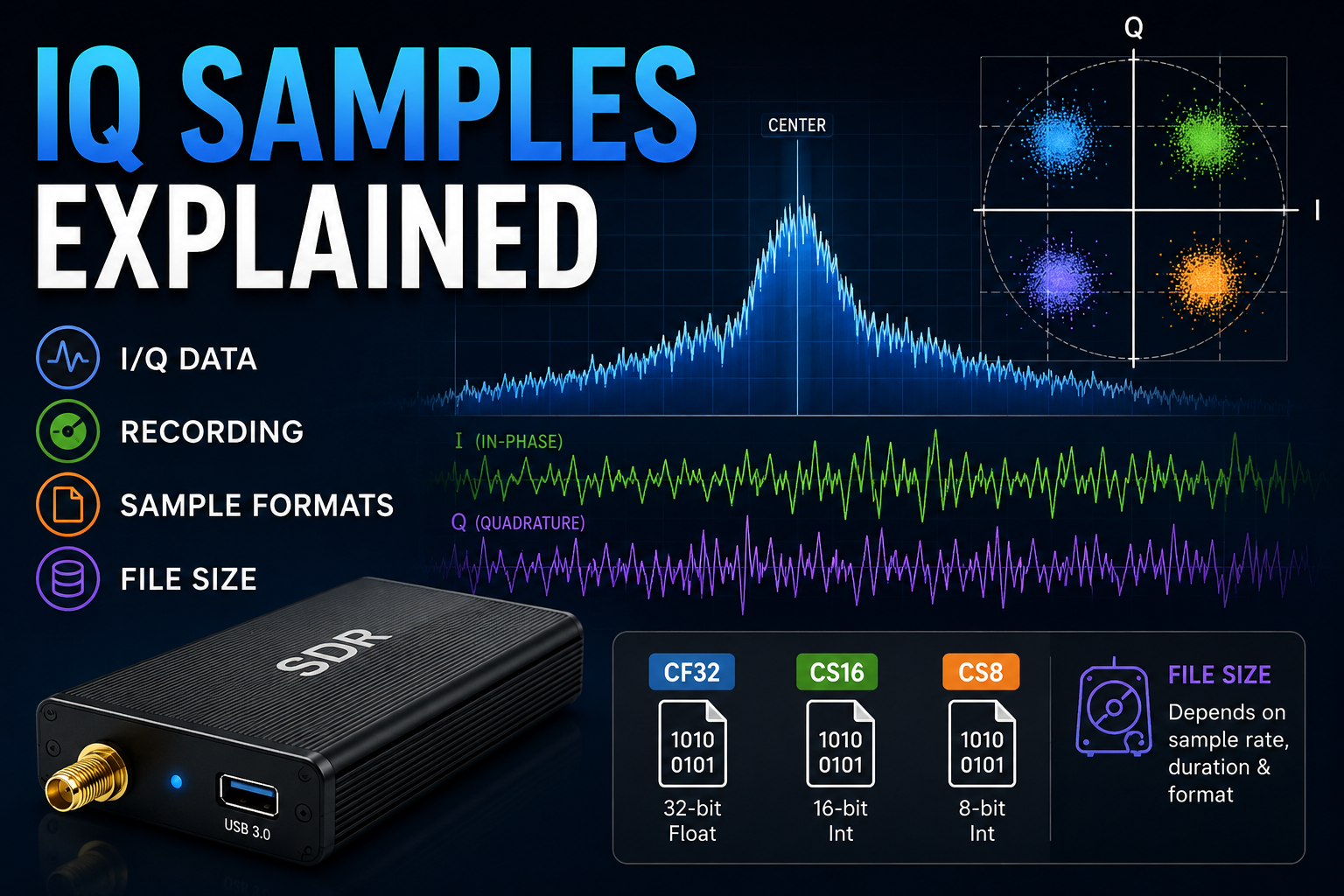
When an SDR records radio spectrum, it normally does not save an MP3, WAV audio track or a list of frequencies.

It records I/Q samples.

Those samples are the digital representation of the radio-frequency signal inside the bandwidth currently being captured. They preserve amplitude and phase information, which means the same recording can later be retuned, filtered, demodulated and analyzed in software.

That flexibility is one of the most powerful features of software-defined radio.

It is also why I/Q recordings can become enormous.

A basic RTL-SDR recording can consume tens of gigabytes per hour. A HackRF recording can exceed 100 GB per hour. Wideband USRP recordings can reach hundreds of megabytes per second or even terabytes per hour depending on sample rate, channel count and sample format.

This guide explains what I and Q actually mean, why SDRs use complex samples, how sample rate relates to bandwidth, the difference between formats such as CU8, CI16, SC16 and CF32, how raw I/Q files are arranged, how SigMF solves metadata problems, and how to calculate SDR recording size before filling an SSD.

What Are I/Q Samples?

I/Q samples are pairs of numbers representing a radio signal in complex baseband.

The two components are:

• I — In-phase
• Q — Quadrature

They can be written mathematically as:

x[n] = I[n] + jQ[n]

where:

• I[n] is the real or in-phase component;
• Q[n] is the imaginary or quadrature component;
• j represents √−1 in electrical engineering notation;
• n is the sample index.

One I value and one Q value together form one complex sample.

I/Q Samples Explained in One Table

Term	Meaning
I	In-phase component of the complex signal
Q	Quadrature component, 90° relative mathematical axis
Complex sample	One I value plus one Q value
Sample rate	Number of complex samples produced each second
Center frequency	RF frequency mapped to 0 Hz in complex baseband
Sample format	How I and Q values are numerically represented and stored
Bit depth	Number of bits used for an individual numerical component
IQ recording	Stored complex baseband samples for later replay or processing

Why Do SDRs Need Both I and Q?

If you kept only one real-valued waveform, positive and negative frequencies around baseband would become difficult to distinguish.

Complex I/Q representation preserves both amplitude and phase information and allows signals above and below the SDR's center frequency to remain mathematically distinct.

This is extremely useful for:

• frequency translation;
• digital filtering;
• AM, FM and phase demodulation;
• QPSK and QAM;
• OFDM;
• radar processing;
• MIMO;
• beamforming;
• direction finding;
• digital modulation analysis;
• spectrum recording.

Why Is Q Called Quadrature?

The mathematical I and Q axes are orthogonal.

An ideal complex sinusoid can be represented as:

I = cos(2πft)

Q = sin(2πft)

The sine and cosine components differ by 90 degrees.

Together they describe a rotating vector in the complex plane.

The amplitude of that vector is:

|x| = √(I² + Q²)

and its phase is:

φ = atan2(Q, I)

This is why I/Q data preserves information that a simple amplitude-only recording would lose.

What Does One Complex Sample Look Like?

Imagine the following sequence:

Sample	I	Q
0	0.70	0.10
1	0.62	0.34
2	0.42	0.57
3	0.15	0.69

Software interprets these as:

0.70 + j0.10

0.62 + j0.34

0.42 + j0.57

0.15 + j0.69

That sequence contains both magnitude and phase information over time.

How I/Q Maps RF Spectrum Around the Center Frequency

Suppose an SDR is tuned to:

100 MHz center frequency

and is recording complex samples at:

2 MSPS

In an ideal complex-sampling model, the digital baseband extends approximately from:

−1 MHz to +1 MHz

relative to the center.

That maps approximately to:

99 MHz to 101 MHz RF

The center frequency maps to complex DC, or 0 Hz in the digital baseband.

Complex baseband	RF frequency with 100 MHz center
−750 kHz	99.25 MHz
−250 kHz	99.75 MHz
0 Hz	100.00 MHz
+250 kHz	100.25 MHz
+750 kHz	100.75 MHz

This ability to distinguish positive and negative baseband frequencies is a major reason SDRs use complex I/Q data.

Sample Rate vs Bandwidth

These terms are related but should not automatically be treated as identical hardware specifications.

Sample rate

The sample rate describes how many complex samples the SDR delivers per second.

Examples:

• 2.4 MSPS = 2.4 million complex samples per second;
• 10 MSPS = 10 million complex samples per second;
• 20 MSPS = 20 million complex samples per second;
• 61.44 MSPS = 61.44 million complex samples per second.

Instantaneous RF bandwidth

This describes how much useful RF spectrum the complete radio can capture at once.

The usable bandwidth can be lower than the nominal sample rate because of:

• analog filters;
• digital filters;
• anti-alias filtering;
• RFIC architecture;
• USB or Ethernet transport limitations;
• device-specific signal-quality requirements.

Do not assume that an SDR running at 20 MSPS necessarily provides a perfectly flat, useful 20 MHz RF passband.

What Does MSPS Mean?

MSPS means million samples per second.

For normal complex SDR data, one “sample” normally means one complete I/Q pair.

Therefore:

20 MSPS = 20 million I values + 20 million Q values every second

It does not mean 10 million I/Q pairs.

This distinction becomes critical when calculating file size.

ADC Bit Depth Is Not the Same as IQ File Format

This is one of the most common SDR misunderstandings.

An SDR might advertise:

• 8-bit ADC;
• 12-bit ADC;
• 14-bit ADC;
• 16-bit ADC.

That does not automatically tell you how many bytes each recorded sample will occupy on your SSD.

The raw converter output may be:

• packed;
• sign-extended;
• converted into 16-bit integers;
• normalized into 32-bit floats;
• transported in one format but stored in another.

For example, UHD explicitly distinguishes:

• OTW format — the over-the-wire representation used between the USRP and host;
• CPU format — the representation used by software in host memory.

A USRP application can, for example, transport samples using an integer format and process them as 32-bit floating-point complex numbers.

The file size depends on what is actually written to disk, not merely the ADC resolution printed on the SDR specification sheet.

Common I/Q Sample Formats

Format	I component	Q component	Bytes per complex sample
CU8	8-bit unsigned integer	8-bit unsigned integer	2 bytes
CI8 / CS8	8-bit signed integer	8-bit signed integer	2 bytes
CI16 / SC16	16-bit signed integer	16-bit signed integer	4 bytes
CF32 / FC32	32-bit floating point	32-bit floating point	8 bytes
CF64 / FC64	64-bit floating point	64-bit floating point	16 bytes

Naming conventions differ between software ecosystems.

For example:

• SigMF uses names such as cf32_le and ci16_le;
• UHD uses names including fc32, sc16 and sc8;
• HackRF documentation commonly refers to signed 8-bit quadrature samples;
• RTL-SDR raw capture tools commonly use unsigned 8-bit I/Q.

Always confirm the format expected by the specific application rather than assuming similarly named files are compatible.

CU8: 8-Bit Unsigned I/Q

CU8 uses:

• one 8-bit unsigned integer for I;
• one 8-bit unsigned integer for Q.

That gives:

2 bytes per complex sample

Values normally occupy the range:

0 to 255

with the signal centered around approximately the middle of that numerical range.

Raw RTL-SDR output is a common example.

CU8 is extremely storage efficient, which makes it useful for inexpensive receiver recordings.

CI8 or CS8: Signed 8-Bit I/Q

Signed 8-bit I/Q also uses:

2 bytes per complex sample

but each component is interpreted as a signed value.

Great Scott Gadgets specifies normal HackRF operation using 8-bit I and 8-bit Q samples, and hackrf_transfer uses signed 8-bit quadrature data.

Typical numerical range:

−128 to +127

This is one reason raw HackRF recordings remain smaller than an equivalent sample-rate recording converted into complex float32.

CI16 / SC16: Signed 16-Bit Complex Samples

SC16 uses:

• 16 bits for I;
• 16 bits for Q.

Total:

32 bits = 4 bytes per complex sample

This is common in higher-performance SDR transport and recording workflows.

Compared with 8-bit complex data at the same sample rate, SC16 doubles storage and transport requirements.

CF32 / FC32: Complex Float 32

GNU Radio frequently uses complex 32-bit floating-point samples internally.

Each sample contains:

• 32-bit floating-point I;
• 32-bit floating-point Q.

Total:

64 bits = 8 bytes per complex sample

GNU Radio's common gr_complex representation corresponds to this type.

Values are frequently normalized to a range around:

−1.0 to +1.0

although exact scaling depends on the source and software.

Float representation is convenient for DSP because filters, FFTs, demodulators and mathematical operations can work directly on floating-point values.

The trade-off is storage.

A CF32 recording requires:

• 4× as much space as CU8;
• 2× as much space as SC16.

at the same complex sample rate and channel count.

CF64: Do You Need 64-Bit Floating-Point IQ?

Usually not for raw RF recording.

CF64 stores:

• 64-bit float I;
• 64-bit float Q.

That requires:

16 bytes per complex sample

It can be useful in specialized numerical-processing workflows where very high computational precision is important.

For ordinary SDR recording, however, converting an 8-, 12- or 16-bit receiver into 64-bit floating point does not magically recover additional RF information that was never measured by the ADC.

How Are I/Q Samples Stored in a Raw File?

The common layout is interleaved:

I0, Q0, I1, Q1, I2, Q2, I3, Q3...

GNU Radio documents this layout for binary complex files, and SigMF requires the in-phase component first for its standard complex datasets.

For a signed 16-bit recording, the bytes conceptually represent:

[I0 16-bit][Q0 16-bit][I1 16-bit][Q1 16-bit]...

For CF32:

[I0 float32][Q0 float32][I1 float32][Q1 float32]...

I/Q Order Matters

Not every historical SDR tool or proprietary format necessarily uses the same assumptions.

If software expects:

I, Q, I, Q

but a file contains:

Q, I, Q, I

the spectrum may appear mirrored or otherwise incorrect.

Always record:

• I/Q ordering;
• sample format;
• endianness;
• sample rate;
• center frequency.

What Is Endianness?

Endianness describes the byte order used to represent multi-byte numerical values.

Common possibilities are:

• little-endian;
• big-endian.

This matters for 16-bit, 32-bit and 64-bit representations.

A raw file can contain the correct samples but still look like nonsense if software interprets the byte order incorrectly.

SigMF makes this explicit with format names such as:

• cf32_le — complex float32 little-endian;
• cf32_be — complex float32 big-endian;
• ci16_le — complex signed-int16 little-endian.

The Problem With a File Named recording.bin

Suppose somebody gives you:

capture.bin

What does it contain?

You still need to know:

• center frequency;
• sample rate;
• sample format;
• I/Q order;
• endianness;
• number of channels;
• timestamp;
• receiver model;
• gain;
• antenna;
• frequency correction;
• whether samples were dropped.

Without this information, a raw binary recording can become nearly useless months later.

SigMF: A Better Way to Store I/Q Recordings

SigMF — Signal Metadata Format was created to solve exactly this problem.

A SigMF recording normally separates:

• the raw signal dataset;
• structured JSON metadata describing that dataset.

Metadata can identify properties including:

• sample format;
• sample rate;
• center frequency;
• hardware;
• capture time;
• author;
• annotations;
• multiple capture segments.

The current SigMF specification includes types such as:

• cu8;
• ci16_le;
• cf32_le;
• cf64_le.

For research, universities, dataset sharing and machine-learning workflows, storing proper metadata is strongly preferable to keeping undocumented raw binary files.

IQ File Size Formula

The basic uncompressed storage calculation is:

File size = sample rate × bytes per complex sample × channels × recording time

For complex data:

Bytes per complex sample = 2 × bytes per I or Q component

Example: 8-bit I + 8-bit Q

Each component requires 1 byte.

Therefore:

2 bytes per complex sample

Example: 16-bit I + 16-bit Q

Each component requires 2 bytes.

Therefore:

4 bytes per complex sample

Example: 32-bit float I + Q

Each component requires 4 bytes.

Therefore:

8 bytes per complex sample

Quick I/Q File Size Table

Complex format	Bytes/sample	2.4 MSPS	10 MSPS	20 MSPS
8-bit I + 8-bit Q	2	4.8 MB/s	20 MB/s	40 MB/s
16-bit I + 16-bit Q	4	9.6 MB/s	40 MB/s	80 MB/s
32-bit float I + Q	8	19.2 MB/s	80 MB/s	160 MB/s

These figures use decimal MB, where 1 MB = 1,000,000 bytes.

How Large Is One Hour of IQ Data?

Sample rate	Format	Data rate	1 minute	1 hour
2.4 MSPS	8-bit I + Q	4.8 MB/s	0.288 GB	17.28 GB
10 MSPS	8-bit I + Q	20 MB/s	1.2 GB	72 GB
20 MSPS	8-bit I + Q	40 MB/s	2.4 GB	144 GB
20 MSPS	16-bit I + Q	80 MB/s	4.8 GB	288 GB
20 MSPS	CF32	160 MB/s	9.6 GB	576 GB
56 MSPS	SC16	224 MB/s	13.44 GB	806.4 GB
56 MSPS	CF32	448 MB/s	26.88 GB	1.6128 TB
100 MSPS	SC16	400 MB/s	24 GB	1.44 TB

These are theoretical uncompressed payload sizes for one complex channel. File headers, metadata, buffering and filesystem details may add small overhead.

Decimal GB vs GiB

Storage vendors normally use decimal units:

1 GB = 1,000,000,000 bytes

Operating systems may display binary units:

1 GiB = 1,073,741,824 bytes

This is why a calculated 144 GB recording may appear closer to approximately 134 GiB in software using binary units.

RTL-SDR IQ Recording Size

The RTL-SDR Blog V3 USB-C is a useful practical example.

A common stable operating rate is approximately:

2.4 MSPS

Raw RTL-SDR samples are normally unsigned 8-bit I/Q.

That means:

2.4 million samples/s × 2 bytes = 4.8 MB/s

which becomes:

• 288 MB/minute;
• 17.28 GB/hour;
• approximately 414.7 GB/day if recording continuously.

This is why even an inexpensive SDR can fill a drive quickly.

Read the RTL-SDR Setup Guide for Windows for the complete beginner setup workflow.

HackRF Pro IQ Recording Size

Great Scott Gadgets specifies the HackRF Pro for normal operation at up to:

20 million samples per second with 8-bit I and 8-bit Q

At 20 MSPS:

20,000,000 × 2 bytes = 40 MB/s

That equals:

• 2.4 GB/minute;
• 144 GB/hour;
• 1 TB in roughly seven hours of continuous uncompressed capture.

HackRF Pro also introduces additional precision modes, so recording size can change when those modes are used.

For normal HackRF Tools operation, hackrf_transfer uses signed 8-bit quadrature samples.

See the HackRF Pro Setup Guide for current software and GNU Radio setup instructions.

USRP B210 IQ Recording Size

The USRP B210 can provide up to 56 MHz of real-time bandwidth per channel according to its product specification.

However, calculating disk requirements requires knowing the host sample format.

56 MSPS stored as SC16

SC16 requires 4 bytes per complex sample:

56,000,000 × 4 = 224 MB/s

Storage:

• 13.44 GB/minute;
• 806.4 GB/hour.

56 MSPS stored as CF32

CF32 requires 8 bytes per complex sample:

56,000,000 × 8 = 448 MB/s

Storage:

• 26.88 GB/minute;
• 1.6128 TB/hour.

These calculations illustrate theoretical uncompressed disk payload requirements; they do not mean every host computer, USB controller or SSD configuration can sustain every possible recording configuration without dropped samples.

Two-Channel Recording Doubles the Data Again

If the B210 records two channels simultaneously, multiply by two.

For example:

56 MSPS × SC16 × 2 channels

equals:

448 MB/s

or:

1.6128 TB/hour

before filesystem/container overhead.

This is why MIMO and coherent-array recording requires careful host planning.

Read 2×2 MIMO SDR Explained for more information about multi-channel SDR architectures.

Sample Format Can Matter More Than You Expect

Consider one channel sampled at 10 MSPS.

Format	Storage rate	1 hour
CI8 / CU8	20 MB/s	72 GB
CI16 / SC16	40 MB/s	144 GB
CF32	80 MB/s	288 GB
CF64	160 MB/s	576 GB

The RF bandwidth and number of captured time samples can remain the same while the storage requirement changes by a factor of eight.

Does Converting 8-Bit IQ to Float32 Improve the Signal?

No.

It makes processing more convenient, but it cannot recreate information that was lost during original quantization.

If an SDR generated an 8-bit I value, converting that number into a 32-bit float only gives software a higher-precision numerical container for subsequent calculations.

It does not turn an 8-bit ADC into a 32-bit ADC.

This distinction is important when designing archival formats.

You might process data as CF32 but still archive the original integer samples to reduce disk requirements.

Quantization and Dynamic Range

Lower sample precision introduces larger quantization steps.

In an ideal converter, increasing bit depth can represent smaller amplitude differences.

But real SDR performance also depends on:

• effective number of bits;
• noise figure;
• clock quality;
• RF gain;
• front-end linearity;
• ADC noise;
• interference;
• RF filtering.

A nominal 16-bit file format does not guarantee 16 bits of useful RF information.

What Is Clipping in I/Q Data?

Digital samples have a maximum representable amplitude.

If the analog signal exceeds the available converter or processing range, samples saturate.

This is called clipping.

Symptoms include:

• flat-topped I or Q time-domain waveforms;
• many unexpected harmonics;
• intermodulation;
• distorted constellation points;
• a raised noise floor;
• incorrect demodulation.

Saving clipped samples in a higher-precision format cannot repair them.

Gain must be configured correctly before or during acquisition.

What Is DC Offset in an IQ Recording?

Direct-conversion SDR receivers can exhibit a DC component around the center of the complex baseband.

On a spectrum display this can appear as a center spike.

Sources can include:

• LO leakage;
• ADC offset;
• mixer imbalance;
• analog imperfections.

Some SDR hardware and software implement DC-removal algorithms.

HackRF Pro, for example, includes architectural improvements intended to eliminate the prominent DC spike associated with earlier HackRF workflows.

Do not automatically interpret every center-frequency feature as an actual RF signal.

What Is I/Q Imbalance?

An ideal receiver produces I and Q paths with:

• equal amplitude response;
• exact 90-degree quadrature relationship.

Real hardware can exhibit:

• gain mismatch;
• phase error;
• frequency-dependent mismatch.

This can create an unwanted mirrored image of a signal.

Higher-end RFICs and SDR software can include correction mechanisms, but accurate measurement applications should still understand I/Q imbalance.

Why Can You Retune Inside an IQ Recording?

An audio recording normally contains one already-demodulated channel.

An I/Q recording contains the entire captured complex baseband.

Suppose an SDR records 2 MHz of spectrum centered at 145 MHz.

Signals throughout that captured region remain in the file.

When replaying it later, software can:

• select a different signal inside the recording;
• change demodulation mode;
• change receiver bandwidth;
• apply different filters;
• run different decoders;
• inspect the waterfall again.

This makes IQ recording extremely useful for:

• RF troubleshooting;
• satellite research;
• wireless protocol development;
• spectrum monitoring;
• signal-classification research;
• university datasets;
• machine learning.

IQ Recording vs Audio Recording

Feature	IQ recording	Audio recording
Contains RF/baseband spectrum	Yes	No
Contains I and Q	Yes	Normally no
Can retune after recording	Within recorded bandwidth	No
Can change demodulation later	Yes	No
Storage requirement	Large to enormous	Much smaller
Best for research	Yes	Only when demodulated audio is all that is needed

Raw IQ vs WAV IQ

Some SDR applications store I/Q data inside WAV-like containers.

This can be convenient because a WAV header can describe properties such as sample rate and bit depth.

However, an I/Q WAV file should not automatically be treated like ordinary stereo audio.

Software may use:

• left channel for I;
• right channel for Q;
• special metadata conventions;
• non-audio sample rates.

Compatibility depends on the recording application.

Raw Binary vs SigMF

Feature	Raw binary	SigMF
Simple	Excellent	Good
Minimal overhead	Excellent	Excellent
Stores center frequency metadata	No	Yes
Stores sample rate metadata	No	Yes
Stores datatype metadata	No	Yes
Research reproducibility	Poor unless separately documented	Strong
Dataset sharing	Easy to misinterpret	Designed for this purpose

When Should You Use SigMF?

SigMF is particularly valuable for:

• university research;
• published datasets;
• RF machine-learning datasets;
• signal-classification work;
• shared laboratory captures;
• long-term archival;
• multi-team engineering projects.

If a recording may be opened by somebody other than the person who captured it—or by the same engineer six months later—metadata is worth storing.

GNU Radio and IQ Samples

GNU Radio is built around streams of typed samples.

Common signal types include:

• complex float32;
• float32;
• int16;
• int8;
• byte.

Complex Float 32 is one of the most common representations used between DSP blocks.

A typical receive flowgraph might look like:

SDR Source → Complex Filter → Demodulator → Audio

The SDR source produces complex I/Q samples. DSP blocks then operate on that complex stream.

A File Sink can instead store those samples directly to disk.

Why GNU Radio Files Can Become Huge

A standard GNU Radio complex File Sink commonly writes CF32.

That means:

8 bytes per complex sample

At only 2.4 MSPS:

2.4 million × 8 = 19.2 MB/s

or:

69.12 GB/hour

That is four times the raw CU8 storage rate of an RTL-SDR at the same sample rate.

The reason is not that GNU Radio suddenly received four times more RF information. It is because the original integer samples have been converted into a larger floating-point representation.

Can You Reduce IQ File Size?

Yes.

1. Lower the sample rate

If you only need a 200 kHz signal, recording 20 MHz of spectrum may be unnecessary.

Filter and decimate before writing to disk.

2. Use a smaller integer format

If the original receiver resolution supports it and the software workflow allows it, storing integer samples can use far less space than CF32.

3. Record only the required channels

A 4-channel coherent receiver uses four times the storage of one channel at the same sample rate and format.

4. Record only when activity is present

Triggered capture can dramatically reduce storage for intermittent signals.

5. Channelize first

Instead of storing a 100 MHz-wide spectrum, extract only the subchannels required by the experiment.

6. Use appropriate compression

Lossless compression may help in some datasets, although noise-like high-entropy RF data often compresses poorly.

Lossy compression should only be used when the research objective allows modification of the samples.

Should You ZIP an IQ File?

You can, but do not expect results similar to compressing text documents.

Real RF captures often contain significant noise entropy.

Noise-like data is difficult to compress losslessly because consecutive values do not contain the predictable redundancy found in text or simple images.

Compression ratios vary greatly depending on:

• signal occupancy;
• sample precision;
• noise level;
• format;
• compression algorithm.

Do not design a storage system around an assumed compression ratio until you have tested representative recordings.

Can You Record Directly to an HDD?

It depends on the sustained data rate.

A slow hard disk might handle a low-rate RTL-SDR capture but struggle with high-rate wideband recordings.

For high-throughput SDR recording, NVMe SSDs are usually more appropriate.

Recording	Approx. write requirement
RTL-SDR 2.4 MSPS CU8	4.8 MB/s
HackRF 20 MSPS CI8	40 MB/s
20 MSPS SC16	80 MB/s
20 MSPS CF32	160 MB/s
56 MSPS SC16	224 MB/s
56 MSPS CF32	448 MB/s

Do not select storage from its advertised peak sequential-write number alone.

For long SDR captures, consider:

• sustained write speed after cache exhaustion;
• thermal throttling;
• free-space availability;
• filesystem overhead;
• simultaneous processing load;
• RAID configuration;
• SSD endurance.

Why SSD Endurance Matters

Wideband RF data can write tens or hundreds of terabytes surprisingly quickly.

A research lab repeatedly recording terabytes of IQ data can consume a significant portion of an SSD's rated write endurance.

For continuous acquisition, check:

• TBW rating;
• enterprise vs consumer workload design;
• thermal cooling;
• power-loss requirements;
• RAID/redundancy strategy.

Dropped Samples Can Ruin a Recording

If the SDR produces samples faster than the host can receive, process or store them, buffers can overflow.

The resulting recording may contain discontinuities.

Common causes include:

• USB bandwidth limitations;
• network packet loss;
• slow storage;
• CPU overload;
• insufficient buffers;
• another application heavily using the disk;
• thermal throttling;
• poor USB cables;
• incorrect NIC tuning.

For casual listening this may only cause a brief glitch.

For radar, coherent processing, protocol research or time-sensitive datasets, a missing block of samples can invalidate an experiment.

Always Store Recording Metadata

At minimum, keep:

• center frequency;
• sample rate;
• sample format;
• endianness;
• I/Q ordering;
• channel count;
• receiver model;
• receiver gain;
• timestamp;
• antenna;
• frequency correction;
• clock source;
• software version;
• whether sample loss occurred.

For research projects, also document:

• RF cables;
• filters;
• LNAs;
• GPS location where appropriate;
• external reference clocks;
• experiment configuration;
• legal/ethical data-handling requirements.

IQ Samples for MIMO and Coherent Receivers

Multi-channel SDR systems increase both the value and complexity of I/Q data.

A coherent 4-channel receiver produces:

I0/Q0 + I1/Q1 + I2/Q2 + I3/Q3

for every sample instant.

If one channel requires 200 MB/s, four channels require approximately:

800 MB/s

before additional overhead.

For coherent research, metadata must also preserve:

• channel ordering;
• sample alignment;
• clock source;
• time source;
• phase-calibration information.

This is important for:

• MIMO;
• beamforming;
• direction finding;
• passive radar;
• channel sounding;
• radio astronomy;
• array processing.

Read Passive Radar with SDR: Hardware, Coherent Receivers, Antennas, and Real-World Research for a practical coherent-recording use case.

IQ Data for Machine Learning

Machine-learning RF projects often use raw or processed I/Q windows as model input.

Possible applications include:

• modulation classification;
• signal detection;
• RF fingerprinting;
• spectrum occupancy classification;
• interference classification;
• neural receiver research.

For reproducible datasets, researchers should document:

• sample rate;
• center frequency;
• sample normalization;
• format;
• window length;
• gain;
• signal labels;
• SNR methodology;
• train/test partitioning.

SigMF can be particularly useful when distributing RF datasets among teams.

How Many IQ Samples Are in a File?

If you know the file size and complex format:

Number of samples = file size in bytes / bytes per complex sample

Example:

A raw 8 GB CF32 file contains:

8,000,000,000 / 8 = 1,000,000,000 complex samples

At 10 MSPS, that represents:

100 seconds of recording

How Long Will My SSD Record?

You can rearrange the file-size formula:

Recording time = available bytes / data rate

Example: 1 TB available, HackRF at 20 MSPS CI8

Data rate:

40 MB/s

Approximate time:

1,000,000 MB / 40 MB/s = 25,000 seconds

or roughly:

6.94 hours

Real usable duration will be lower because the drive should not normally be filled completely and filesystem/application overhead may apply.

Common IQ Recording Mistakes

1. Forgetting the sample format

A raw file without format information may be impossible to interpret correctly later.

2. Forgetting the sample rate

The playback software cannot correctly map digital frequencies or time without it.

3. Forgetting the center frequency

The I/Q file contains baseband offsets, not enough information by itself to reconstruct absolute RF frequencies.

4. Confusing ADC bit depth with disk format

A 12-bit SDR may still produce a 16-bit or float32 host recording.

5. Calculating only one component

Remember that complex samples contain both I and Q.

6. Forgetting channel count

Two-channel MIMO doubles storage. Four channels quadruple it.

7. Recording an unnecessarily high sample rate

Filter and decimate if only a narrow signal is needed.

8. Using a slow SSD or HDD

A benchmark showing high burst speed does not guarantee long sustained capture performance.

9. Filling the operating-system drive

Running out of disk space during an experiment can crash applications and create corrupted captures.

10. Ignoring dropped samples

A file can have the expected size while still containing timing discontinuities.

Which SDR Is Best for IQ Recording?

The correct SDR depends on how much spectrum you need to capture.

SDR class	Recording strength	Main consideration
RTL-SDR Blog V3 USB-C	Low-cost narrowband recordings	Small sample rate keeps storage manageable
HackRF Pro	Wideband 8-bit IQ capture up to 20 MSPS in normal mode	About 144 GB/hour at maximum normal rate
PLUTO+	Networked/USB SDR experiments and multi-channel workflows	Actual host bandwidth and firmware configuration matter
bladeRF 2.0 micro xA9	High-rate USB 3.0 and FPGA-oriented research	High sample rates demand fast host storage
USRP B210	Professional dual-channel wideband IQ research	Format and two-channel operation can produce enormous datasets

Browse software-defined radio hardware at SDRstore.eu for additional receiver and transceiver options.

Which Software Should You Use for IQ Recording?

SDR++

Good for interactive receiving, waterfall use and general-purpose recording workflows with many SDRs.

SDRSharp

Popular on Windows, particularly with RTL-SDR and plugin-based receiver workflows.

SDRangel

Useful for more advanced receive/transmit and channel-processing configurations.

GNU Radio

Best when you need complete control over:

• sample format;
• decimation;
• filtering;
• metadata;
• multi-channel acquisition;
• custom DSP;
• network streaming.

Read Best SDR Software in 2026 or SDR++ vs SDRSharp vs SDRangel for software comparisons.

Buyer Advice: Plan Storage Before Buying a Wideband SDR

A buyer may see “56 MHz bandwidth” or “100 MHz bandwidth” and assume the only requirement is a fast SDR.

The SDR may actually be the easiest part.

A complete wideband recording system must support:

• SDR data rate;
• USB, Ethernet or PCIe throughput;
• CPU memory movement;
• sample-format conversion;
• sustained SSD write rate;
• available capacity;
• SSD endurance;
• backup/archival strategy.

Before purchasing hardware, calculate:

sample rate × sample size × channel count × required duration

Then design the host around that number.

For Universities, RF Labs and Research Teams

Universities, research laboratories, telecom companies, cybersecurity firms, AI/ML research teams and engineering organizations can request quotations for complete SDR acquisition and recording systems through SDRstore.eu.

Use the Add to Quote button on individual product pages or the document icon on product cards while browsing.

A complete IQ recording setup can include:

• RTL-SDR receivers;
• HackRF Pro;
• bladeRF;
• USRP B210;
• networked USRP platforms;
• antennas;
• RF filters;
• attenuators;
• clocking hardware;
• RF test equipment;
• other hardware required for the research bench.

This is particularly useful when designing RF dataset-generation systems, signal-classification labs, MIMO experiments and university GNU Radio laboratories.

Recommended Workflow for Research IQ Recordings

1. Define the minimum required RF bandwidth.
2. Select a sample rate with appropriate filter margin.
3. Choose the SDR.
4. Select the raw or processed sample format.
5. Calculate bytes per second.
6. Multiply by channel count.
7. Calculate total experiment duration.
8. Choose storage with sufficient sustained write speed.
9. Record metadata using SigMF or equivalent documentation.
10. Test for dropped samples before the real experiment.
11. Capture a short validation file.
12. Replay that file in the intended analysis software.
13. Only then begin long-duration acquisition.

Official Technical References

• SigMF — Signal Metadata Format Specification
• GNU Radio — Signal Data Types
• GNU Radio — Reading and Writing Binary Files
• UHD Manual — Device Streaming and Sample Data Types
• UHD Manual — Sample Format Converters
• Great Scott Gadgets — HackRF Pro
• Great Scott Gadgets — HackRF Tools

Final Recommendation

The most important thing to understand about SDR I/Q data is that one complex sample contains both an I value and a Q value.

That single fact explains why file-size calculations often surprise new SDR users.

The basic formula is:

sample rate × bytes per complex sample × channel count × recording time

Remember:

• 8-bit I + 8-bit Q = 2 bytes/sample;
• 16-bit I + 16-bit Q = 4 bytes/sample;
• CF32 = 8 bytes/sample;
• CF64 = 16 bytes/sample.

A 2.4 MSPS RTL-SDR CU8 recording is approximately 17.28 GB/hour.

A normal 20 MSPS HackRF 8-bit I/Q recording is approximately 144 GB/hour.

A hypothetical one-channel 56 MSPS SC16 recording is approximately 806.4 GB/hour.

The same 56 MSPS samples stored as CF32 become approximately 1.61 TB/hour.

For multi-channel SDRs, multiply again by the number of recorded channels.

Finally, do not archive undocumented capture.bin files. Preserve sample rate, center frequency, datatype, endianness, receiver settings and acquisition metadata. For serious research and dataset sharing, use SigMF or an equally rigorous metadata workflow.

FAQ

What are I/Q samples?

I/Q samples are pairs of in-phase and quadrature values representing a signal as complex baseband data. Together they preserve both amplitude and phase information for SDR processing.

Is one I/Q pair one sample?

Yes. In normal complex SDR terminology, one complex sample contains one I value and one Q value. Therefore 10 MSPS normally means 10 million I/Q pairs per second.

Why do SDRs use I and Q?

I/Q representation preserves amplitude and phase and allows positive and negative frequencies around the tuned center frequency to be represented independently. This makes digital tuning, filtering, modulation and demodulation practical.

How large is an IQ recording?

Multiply sample rate by bytes per complex sample, number of channels and recording duration. For example, 20 MSPS with 8-bit I and 8-bit Q requires 40 MB/s or approximately 144 GB per hour for one channel.

How many bytes is one complex float32 sample?

A complex float32 sample contains a 32-bit floating-point I component and a 32-bit floating-point Q component, for a total of 64 bits or 8 bytes per complex sample.

How many bytes is SC16 IQ?

SC16 uses one signed 16-bit integer for I and one signed 16-bit integer for Q, giving 32 bits or 4 bytes per complex sample.

What is CU8 IQ?

CU8 is complex unsigned 8-bit data. I uses one unsigned byte and Q uses one unsigned byte, giving 2 bytes per complex sample. Raw RTL-SDR recordings commonly use this representation.

What sample format does HackRF use?

Normal HackRF streaming uses 8-bit I and 8-bit Q samples. Great Scott Gadgets documents hackrf_transfer files as signed 8-bit quadrature samples.

Does converting 8-bit IQ to float32 improve receiver resolution?

No. Float32 can make subsequent DSP calculations more convenient and precise, but it cannot recover RF information that was not captured by the original converter.

Is sample rate the same as RF bandwidth?

Not necessarily. Complex sample rate establishes the digital sampling space, but usable instantaneous RF bandwidth also depends on analog and digital filters, RFIC design and the SDR's host interface.

What is a SigMF file?

SigMF is a standardized way to describe recorded signal datasets. It stores metadata such as sample format, sample rate and capture information alongside the raw signal dataset so recordings can be interpreted and shared reliably.

What is the difference between FC32 and SC16?

FC32 stores each I and Q component as a 32-bit floating-point number and requires 8 bytes per complex sample. SC16 stores each component as a signed 16-bit integer and requires 4 bytes per complex sample.

Why are GNU Radio IQ recordings so large?

GNU Radio commonly processes complex float32 data, which requires 8 bytes per complex sample. A 2.4 MSPS CF32 recording therefore requires approximately 19.2 MB/s or 69.12 GB per hour.

How can I reduce IQ recording size?

Reduce the sample rate, filter and decimate before recording, store an appropriate integer format, record fewer channels, use triggered acquisition or extract only the subchannel you actually need.

Can I compress IQ recordings?

Yes, but lossless compression ratios can be poor because RF noise has high entropy. Test representative recordings before relying on compression for storage planning.

What SSD speed do I need for IQ recording?

Your sustained disk write speed must exceed the complete IQ data rate with additional margin. For example, one 56 MSPS SC16 channel produces approximately 224 MB/s before overhead, while CF32 at the same sample rate produces approximately 448 MB/s.

Do two SDR channels double file size?

Yes. If both channels use the same sample rate and format, two channels produce twice as much data as one. Four channels produce four times as much.

What metadata should I save with IQ data?

At minimum save center frequency, sample rate, datatype, endianness, I/Q order, channel count, timestamp, SDR model and gain settings. Research projects should also document antennas, clocks, filters and other acquisition details.